Indices of diversity from NDVI.

require(rasterdiv)
require(rasterVis)
require(RColorBrewer)

This vignette uses rasterdiv to build global series of indices of diversity based on Information Theory. The input dataset is the Copernicus Long-term (1999-2017) average Normalised Difference Vegetation Index for the 21st of June (copNDVI).

Overview

A RasterLayer called copNDVI is loaded together with the package rasterdiv. copNDVI is a 8-bit raster, meaning that pixel values range from 0 to 255. You could stretch it to match a more familiar (-1,1) values range using raster::stretch(copNDVI,minv=-1,maxv=1) .

Reclassify NDVI

Pixels with values 253, 254 and 255 (water) will be set as NA’s.

copNDVI <- raster::reclassify(copNDVI, cbind(252,255, NA), right=TRUE)

Resample NDVI to a coarser resolution

To speed up the calculation, the RasterLayer will be “resampled” at a resolution 10 times coarser than original and cut on Africa.

#Resample using raster::aggregate and a linear factor of 20
copNDVIlr <- raster::aggregate(copNDVI, fact=30)
#Set float numbers as integers to further speed up the calculation
storage.mode(copNDVIlr[]) = "integer"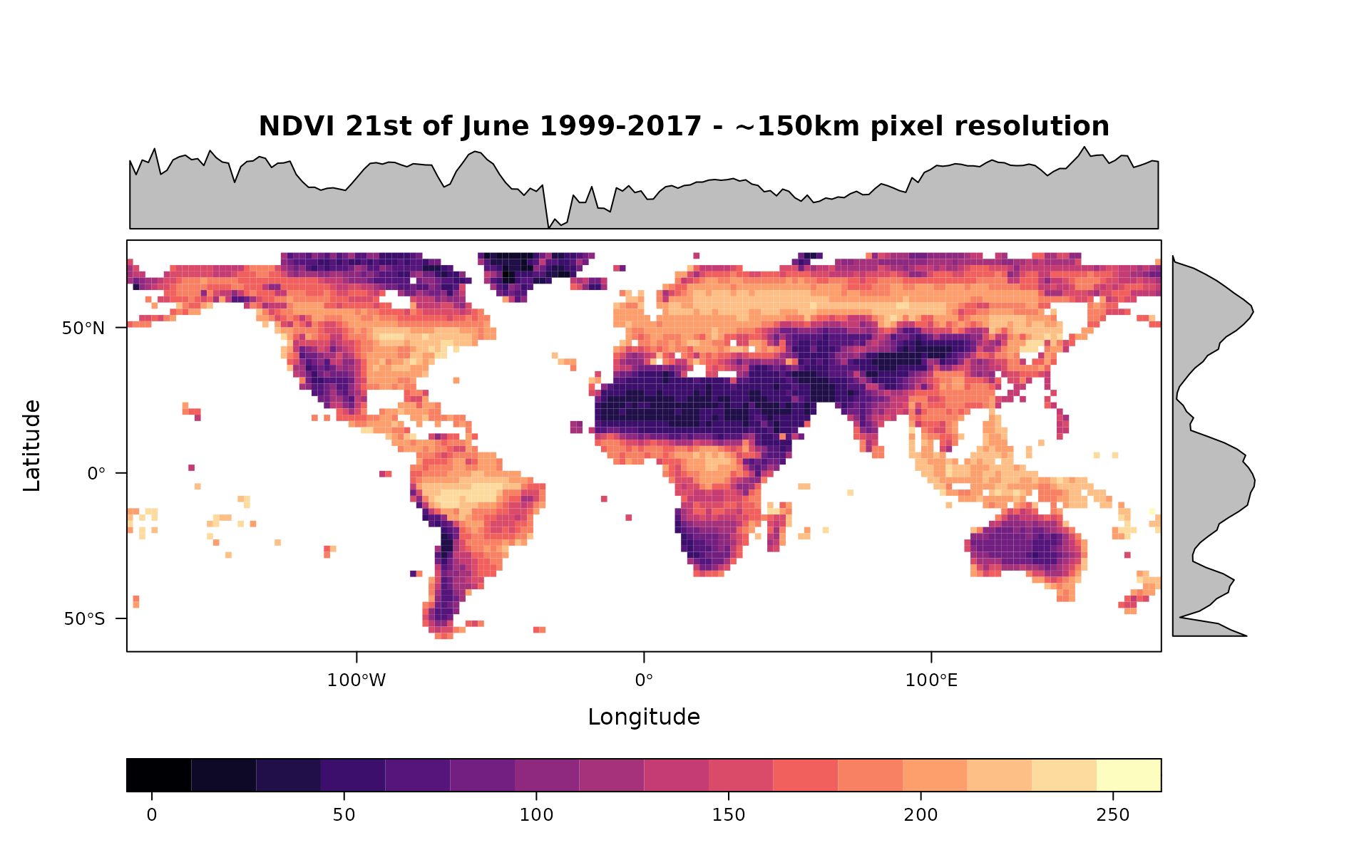

Show resampled NDVI data

levelplot(copNDVIlr,layout=c(0,1,1), main="NDVI 21st of June 1999-2017 - ~150km pixel resolution")

Compute all indexes in rasterdiv

rasterdiv allows the computation of 8 diversity indexes based on information theory. In the following section, all these indexes will be computed for copNDVIlr using a moving window of 81 pixels (9 px side). Alpha values for the Hill, Rényi and parametric Rao indexes will be set from 0 to 2 every 0.5. In addition, we will set na.tolerance=0.1, meaning that all moving windows with more than 10% of pixels equal NA will be set to NA.

#Shannon's Diversity
sha <- Shannon(copNDVIlr,window=9,na.tolerance=0.2,np=1)

#Pielou's Evenness
pie <- Pielou(copNDVIlr,window=9,na.tolerance=0.2,np=1)

#Berger-Parker's Index
ber <- BergerParker(copNDVIlr,window=9,na.tolerance=0.2,np=1)

#Parametric Rao's quadratic entropy with alpha ranging from 1 to 5
prao <- paRao(copNDVIlr, window=9, alpha=1:3, na.tolerance=0.2, dist_m="euclidean",np=1)

#Cumulative Residual Entropy
cre <- CRE(copNDVIlr,window=9,na.tolerance=0.2, np=1)

#Hill's numbers
hil <- Hill(copNDVIlr,window=9,alpha=seq(0,1,0.5),na.tolerance=0.2,np=1)

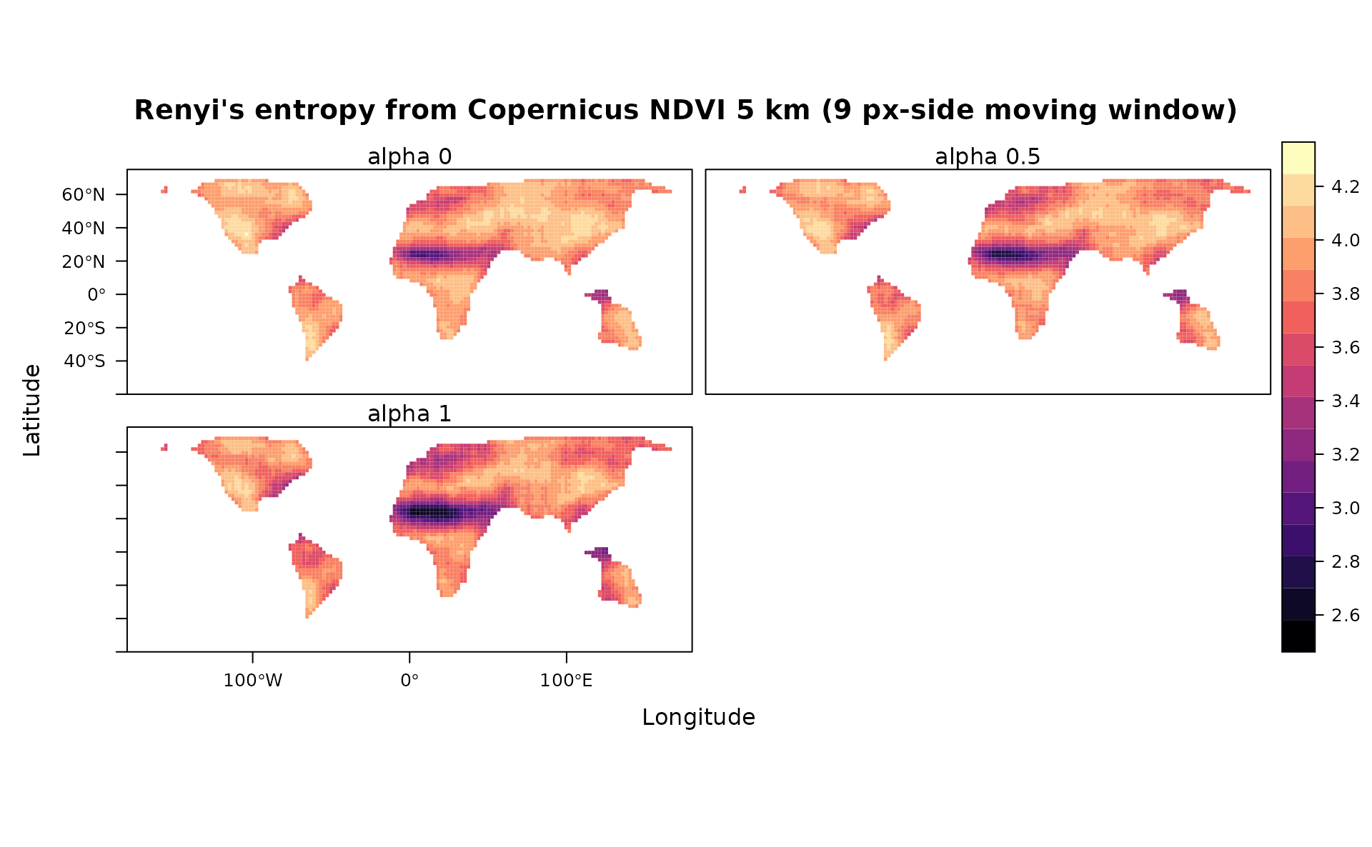
#Rényi's Index
ren <- Renyi(copNDVIlr,window=9,alpha=seq(0,1,0.5),na.tolerance=0.2,np=1)

Visualise RasterLayers (the shape of continents is deformed by the NAs in the 9x9 moving windows)

#Shannon's Diversity
levelplot(sha,main="Shannon's entropy from Copernicus NDVI 5 km (9 px-side moving window)",as.table = T,layout=c(0,1,1), ylim=c(-60,75), margin = list(draw = TRUE))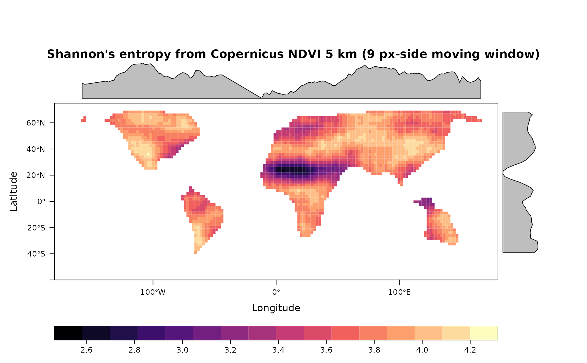

#Pielou's Evenness
levelplot(pie,main="Pielou's evenness from Copernicus NDVI 5 km (9 px-side moving window)",as.table = T,layout=c(0,1,1), ylim=c(-60,75), margin = list(draw = TRUE))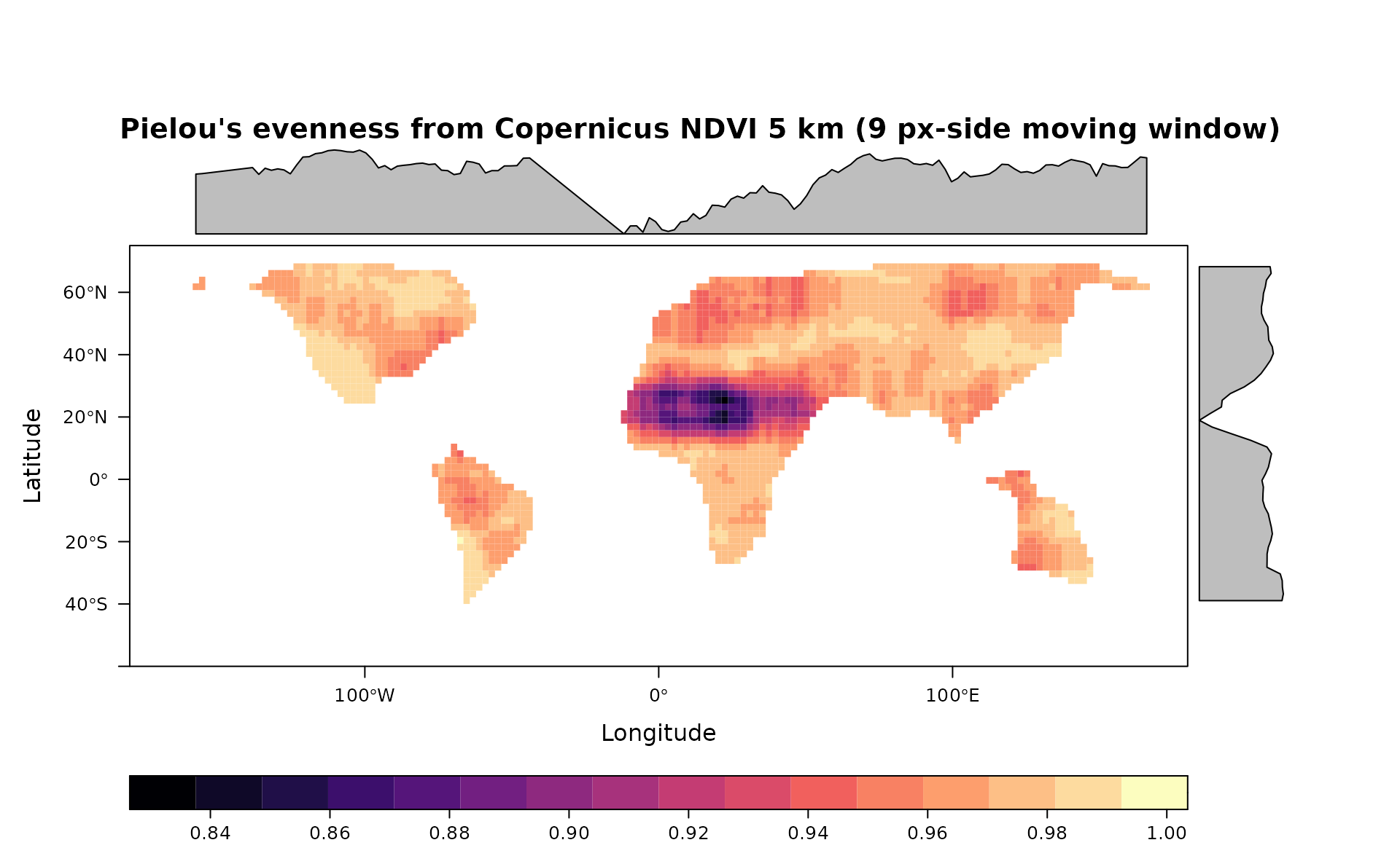

#Berger-Parker' Index
levelplot(ber,main="Berger-Parker's index from Copernicus NDVI 5 km (9 px-side moving window)",as.table = T,layout=c(0,1,1), ylim=c(-60,75), margin = list(draw = TRUE))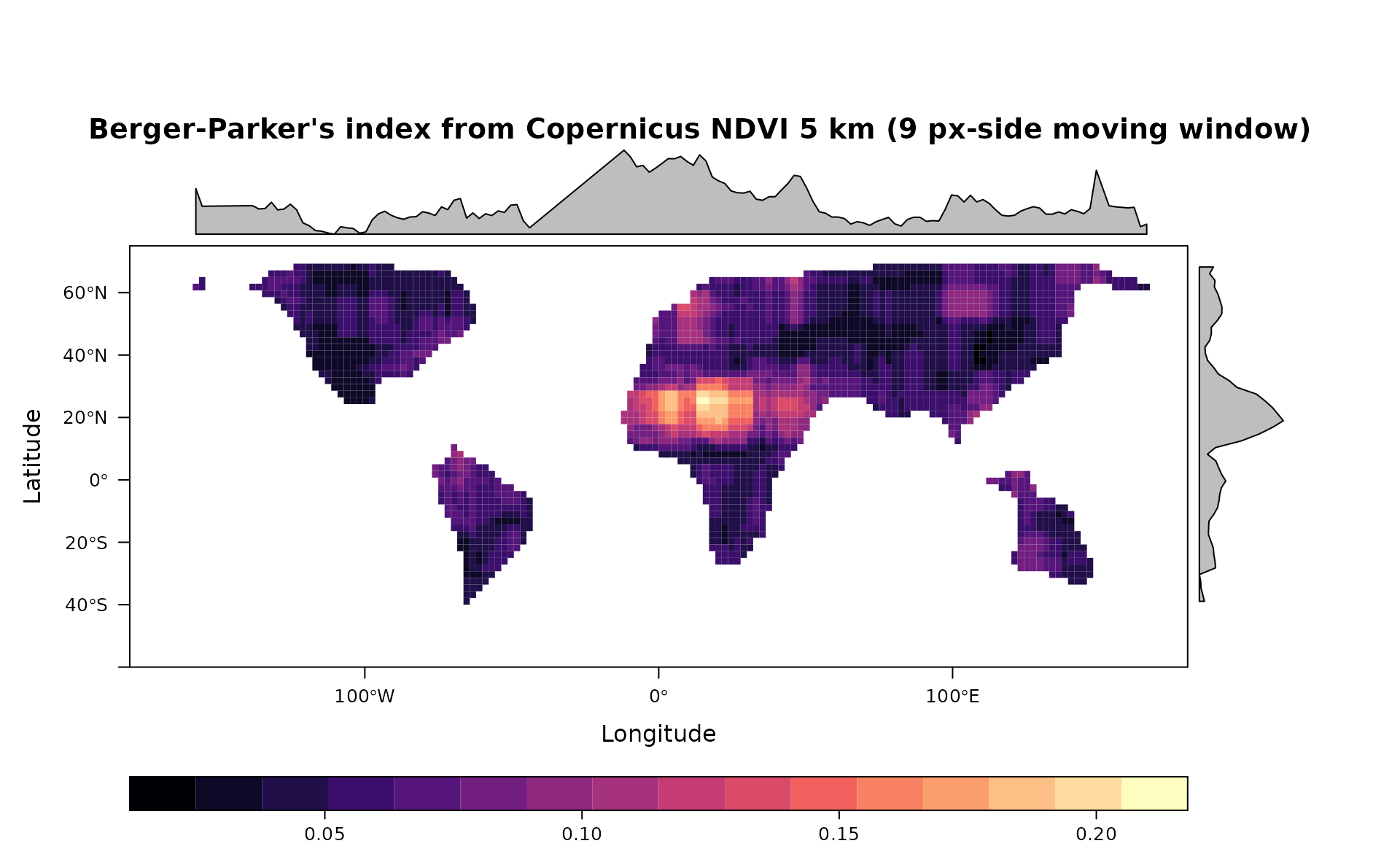

#Parametric Rao's quadratic Entropy
levelplot(stack(prao[[1]]),main="Parametric Rao's quadratic entropy from Copernicus NDVI 5 km (9 px-side moving window)",as.table = T,layout=c(0,3,1), ylim=c(-60,75), margin = list(draw = TRUE))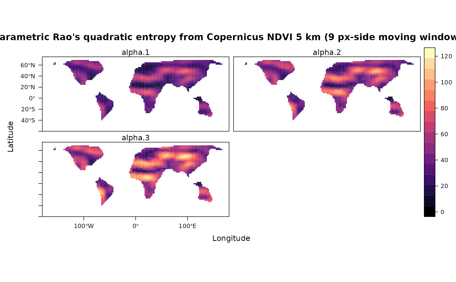

#Cumulative Residual Entropy
levelplot(cre,main="Cumulative Residual Entropy from Copernicus NDVI 5 km (9 px-side moving window)",as.table = T,layout=c(0,1,1), ylim=c(-60,75), margin = list(draw = TRUE))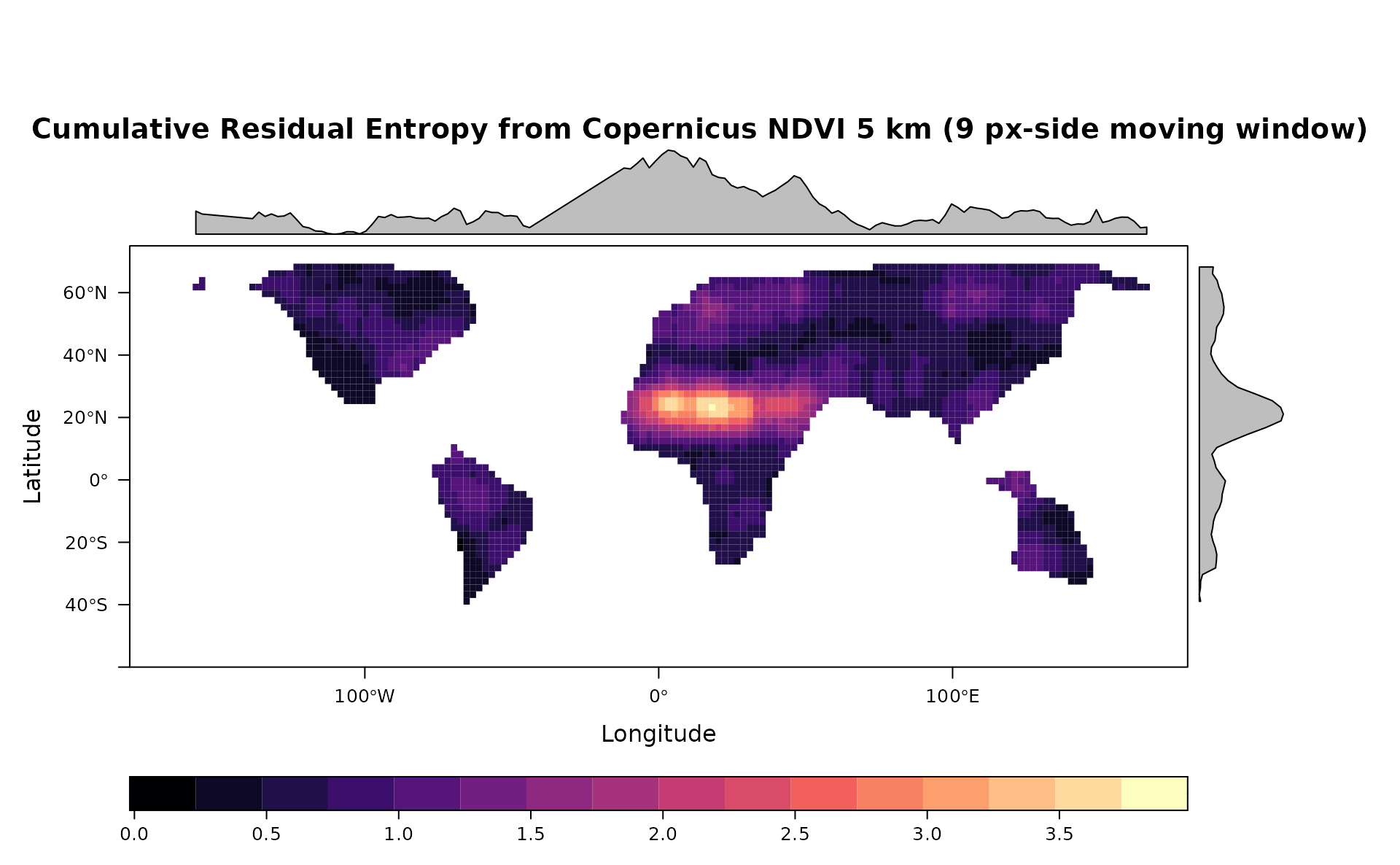

#Hill's numbers (alpha=0, 0.5 and 1)
levelplot(stack(hil),main="Hill's numbers from Copernicus NDVI 5 km (9 px-side moving window)",as.table = T,layout=c(0,3,1), ylim=c(-60,75))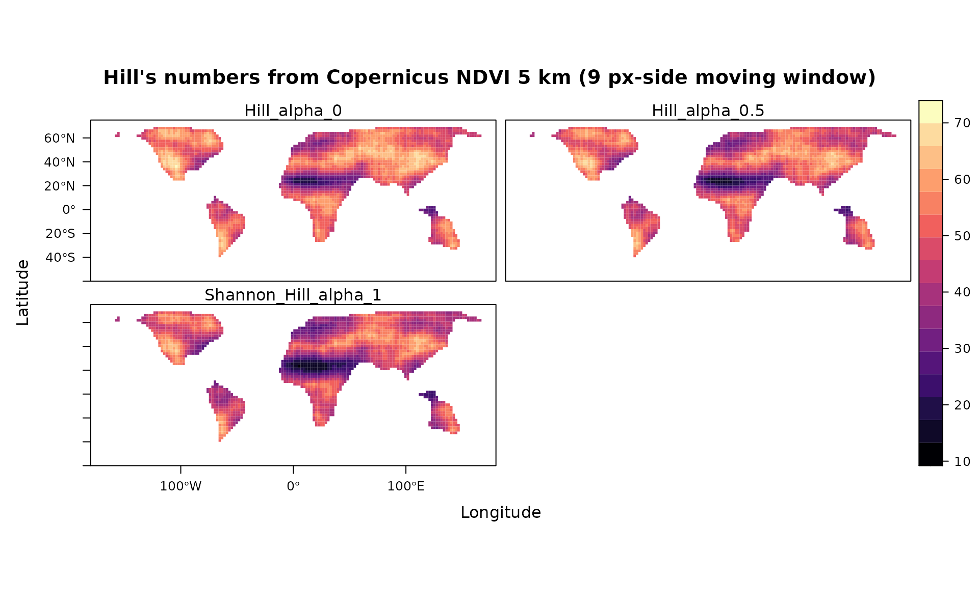

#Renyi' Index (alpha=0, 0.5 and 1)
levelplot(stack(ren),main="Renyi's entropy from Copernicus NDVI 5 km (9 px-side moving window)",as.table = T,layout=c(0,3,1),names.attr=paste("alpha",seq(0,1,0.5),sep=" "), ylim=c(-60,75), margin = list(draw = FALSE))